Recent
Multivariate analysis
El análisis estadístico de alta dimensión y tamaño de muestra pequeño (HDLSS) se está aplicando cada vez más en una amplia gama de contextos. En tales situaciones, se ve que el popular método de la Máquina de Vectores Soporte (SVM) sufre de ''Acumulación de datos'' en el margen, lo que puede disminuir la capacidad de generalización del modelo. Esto conduce al desarrollo de la Distance Weighted Discrimination para encontrar un hiperplano separador . En el presente trabajo se revisa y reproduce, con detalle en la derivación y solución de la función de pérdida que se resuelve usando SOCP, del método desarrollado en e implementado en el entorno R\cite{R}. Basado en el trabajo e implementación de se aplica y comparan resultados a conjuntos de datos reales y simulados (en medida de lo posible los mismos conjuntos de datos utilizados que en) Palabras clave: SVM, kernel, R (el ambiente de cómputo estadístico) y datos de alta dimensión con tamaño de muestra pequeño (data High Dimension Low Sample Size).
A proof is given that the summation of all prime numbers can be assigned the value of 13/12, as well as values that can be assigned to the summation of all multiples and all odd multiples.
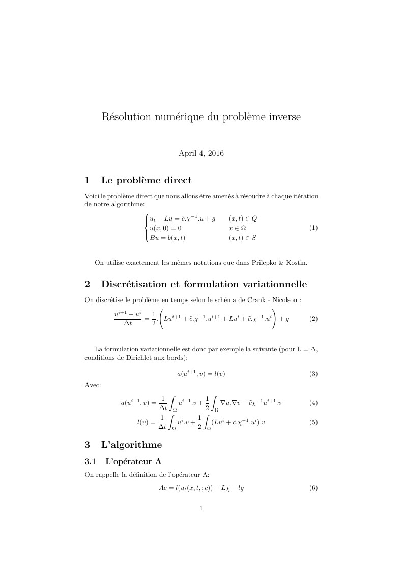
Résolution de problème inverse par point fixe
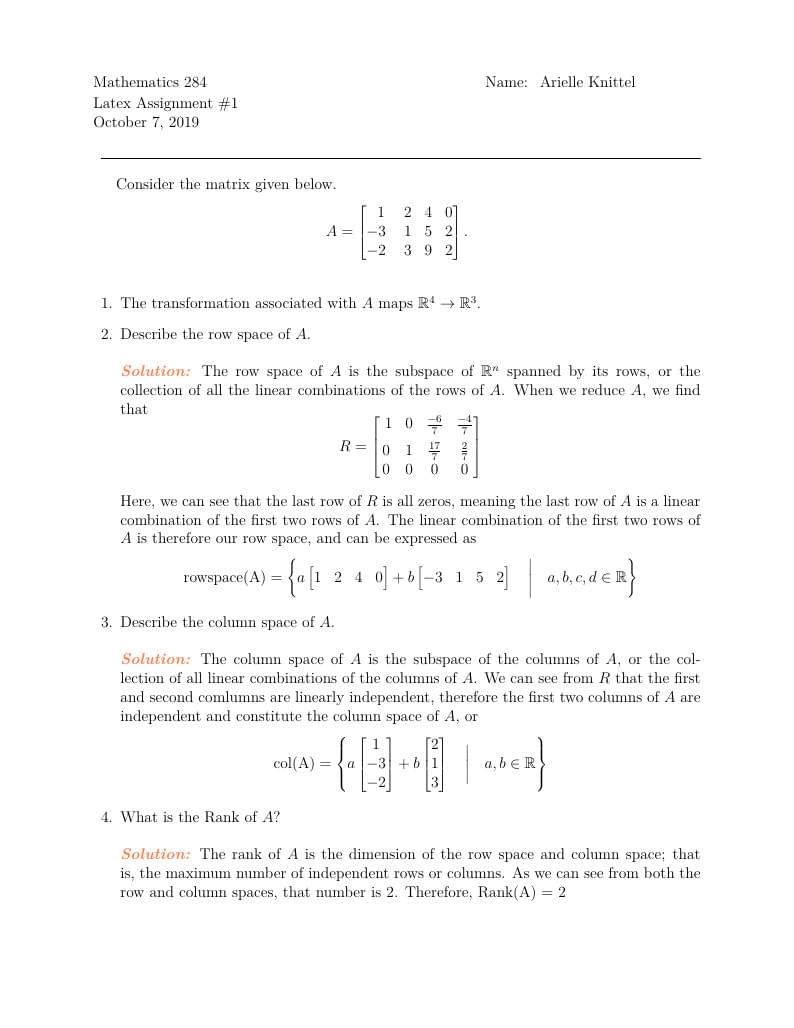
First assignment dealing with nullspace and rowspace
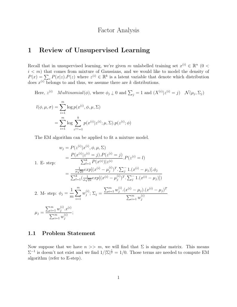
Just another Factor Analysis derivation. Refer to Stanford Lecture Notes CS229.
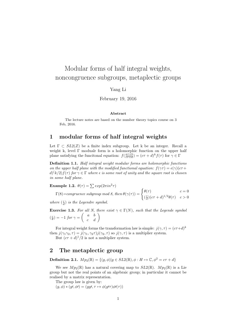
The lecture notes are based on the number theory topics course on 3 Feb, 2016.
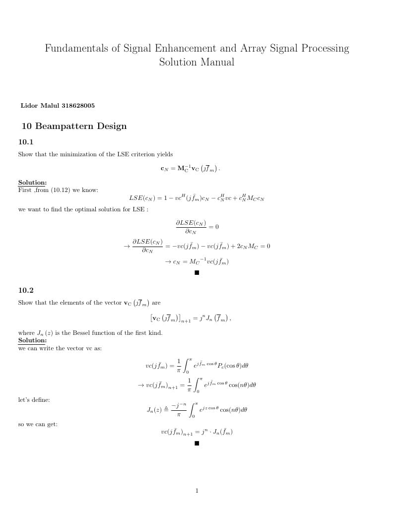
section 10

ÁLGEBRA LINEAL
\begin
Discover why over 25 million people worldwide trust Overleaf with their work.